library(tidyverse)
library(openintro)
library(tidymodels)
library(ggthemes)Inference for two independent means
Warm up
Announcements
- Tomorrow we will talk about final report formatting
- Monday: presentation day
- Wednesday: project report due
Inference for comparing two means
Today’s focus
Inference for comparing two population means
Specifically, making decisions via hypothesis tests
And generally, what in the world is a hypothesis test?!
Different than comparing two paired means:
- Two sets of observations are paired if each observation in one set has a special correspondence or connection with exactly one observation in the other dataset.
Setup
Randomization test for comparing two means
Combine the data from the two groups and randomly shuffle them into two groups of sizes equal to the original group sample sizes
Calculate the means of each group and record the different
Repeat steps 1 and 2 many times to build the null distribution
Find the p-value as the number of simulations with simulated differences at least as extreme (in the direction of the alternative hypothesis) as the observed difference
Case study: Birth weights of babies and smoking
Every year, the United States Department of Health and Human Services releases to the public a large dataset containing information on births recorded in the country. This dataset has been of interest to medical researchers who are studying the relation between habits and practices of expectant mothers and the birth of their children. In this case study we work with a random sample of 1,000 cases from the dataset released in 2014. The distributions of birth weights of babies, measured in pounds, by mother’s smoking habit are shown below.
glimpse(births14)Rows: 1,000
Columns: 13
$ fage <int> 34, 36, 37, NA, 32, 32, 37, 29, 30, 29, 30, 34, 28, 28,…
$ mage <dbl> 34, 31, 36, 16, 31, 26, 36, 24, 32, 26, 34, 27, 22, 31,…
$ mature <chr> "younger mom", "younger mom", "mature mom", "younger mo…
$ weeks <dbl> 37, 41, 37, 38, 36, 39, 36, 40, 39, 39, 42, 40, 40, 39,…
$ premie <chr> "full term", "full term", "full term", "full term", "pr…
$ visits <dbl> 14, 12, 10, NA, 12, 14, 10, 13, 15, 11, 14, 16, 20, 15,…
$ gained <dbl> 28, 41, 28, 29, 48, 45, 20, 65, 25, 22, 40, 30, 31, NA,…
$ weight <dbl> 6.96, 8.86, 7.51, 6.19, 6.75, 6.69, 6.13, 6.74, 8.94, 9…
$ lowbirthweight <chr> "not low", "not low", "not low", "not low", "not low", …
$ sex <chr> "male", "female", "female", "male", "female", "female",…
$ habit <chr> "nonsmoker", "nonsmoker", "nonsmoker", "nonsmoker", "no…
$ marital <chr> "married", "married", "married", "not married", "marrie…
$ whitemom <chr> "white", "white", "not white", "white", "white", "white…Note that there are some NAs in the habit variable.
births14 |>
  count(habit)
# A tibble: 3 × 2
habit n
<chr> <int>
1 nonsmoker 867
2 smoker 114
3 <NA> 19Let’s drop those since we can’t use those observations in our analysis.
births14 <- births14 |>
  drop_na(habit)
births14 |>
ggplot(aes(x = weight, color = habit, fill = habit)) +
geom_density(alpha = 0.5)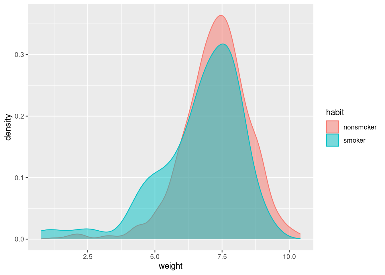
Randomization test for comparing two means
Exercise 1
Set the hypotheses for testing if there is a difference between mean birth weight of babies born to mothers who are smokers and those born to mothers who are not smokers.
\(H_0: \mu_{ns} = \mu_{s}\); the mean weight of babies in the non smoker and smoker groups are the same.
\(H_A: \mu_{ns} \neq \mu_{s}\); the mean weights are different.
Exercise 2
Calculate the observed difference between the mean birth weight of babies born to mothers who are smokers and those born to mothers who are not smokers in this sample.
obs_stat <- births14 |>
  specify(response = weight, explanatory = habit) |>
  calculate(stat = "diff in means", order = c("nonsmoker", "smoker"))
obs_stat
Response: weight (numeric)
Explanatory: habit (factor)
# A tibble: 1 × 1
stat
<dbl>
1 0.593births14 |>
group_by(habit) |>
summarise(mean_weight = mean(weight))# A tibble: 2 × 2
habit mean_weight
<chr> <dbl>
1 nonsmoker 7.27
2 smoker 6.68Exercise 3
Suppose the birth weights of the babies in this sample are written on pieces of paper. Explain how you would conduct the randomization test tactically.
Add answer here.
Exercise 4
Construct and visualize the null distribution. Based on your visualization, speculate on whether the p-value will be small or large.
set.seed(1234)

null_dist <-  births14 |>
  specify(response = weight, explanatory = habit) |>
  hypothesise(null = "independence") |>
  generate(reps = 1000, type = "permute") |>
  calculate(stat = "diff in means", order = c("nonsmoker", "smoker"))

null_dist |>
  visualize()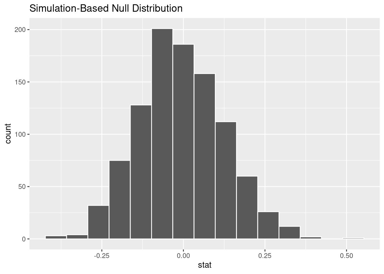
On this histogram, we don’t obseve any values as extreme as our observed statistic of 0.59, so we expect the p-value to be nearly 0.
Exercise 5
Visualize and calculate the p-value. At the 5% discernability level, what is the conclusion of the hypothesis test?
null_dist |>
  get_p_value(obs_stat = obs_stat, direction = "two sided")
Warning: Please be cautious in reporting a p-value of 0. This result is an approximation
based on the number of `reps` chosen in the `generate()` step.
ℹ See `get_p_value()` (`?infer::get_p_value()`) for more information.# A tibble: 1 × 1
p_value
<dbl>
1 0null_dist |>
visualize() +
shade_p_value(obs_stat = obs_stat, direction = "two sided")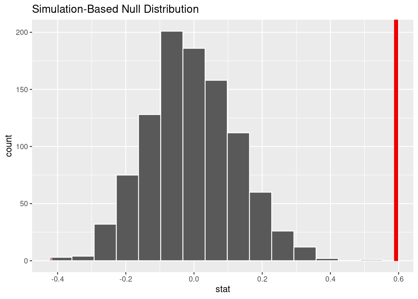
The p-value is close to 0 and smaller than discernability level of 0.05, so reject the null hypothesis. We have sufficient evidence that there is a difference between mean birth weight of babies born to mothers who are smokers and those born to mothers who are not smokers.
Bootstrap interval for the difference of two means
Exercise 6
Construct and interpret confidence interval at the equivalent level as the previous hypothesis test for the difference between the mean weight of babies born to mothers who are not smokers and those who are born to mothers who are smokers.
boot_dist <- births14 |>
  specify(response = weight, explanatory = habit) |>
  generate(reps = 1000, type = "bootstrap") |>
  calculate(stat = "diff in means", order = c("nonsmoker", "smoker"))

ci <- boot_dist |>
  get_ci()

ci
# A tibble: 1 × 2
lower_ci upper_ci
<dbl> <dbl>
1 0.308 0.900visualize(boot_dist) +
shade_ci(ci)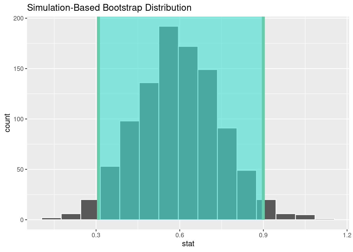
Inference using mathematical models for comparing two means
The two conditions necessary to model the difference in sample means using \(t\)-distribution are: - Independent observations both, within and between samples. - Large sample size in each group and no extreme outliers.
When null hypothesis is true and the conditions are met, we can use a \(t\)-distribution with \(df = \min(n_1-1, n_2-1)\).
Mathematical model for estimating the difference in means using confidence intervals
The \(t\)-distribution can be used for inference when working with the standardized difference of two means if - The data are independent within and between the two groups - We check the outliers for each group separately.
Then, the margin or error is \(t^*_{df}\times \sqrt{\frac{s_1^2}{n_1} - \frac{s_2^2}{n_2}}\).
Exercise 7
Check that the technical conditions for conducting inference using mathematical models for comparing two means are met for these data.
Independent observations within and between groups and 114 and 867 are both large.
Exercise 8
Conduct a hypothesis test using mathematical models for the hypotheses you set in Section 3.1.
t_hat <- births14 |>
  specify(response = weight, explanatory =  habit) |>
  calculate("t", order = c("nonsmoker", "smoker"))

null_dist_theory <- births14 |>
  specify(response = weight, explanatory =  habit)|>
  assume("t")

visualise(null_dist_theory) +
  shade_p_value(obs_stat = t_hat, direction = "two-sided")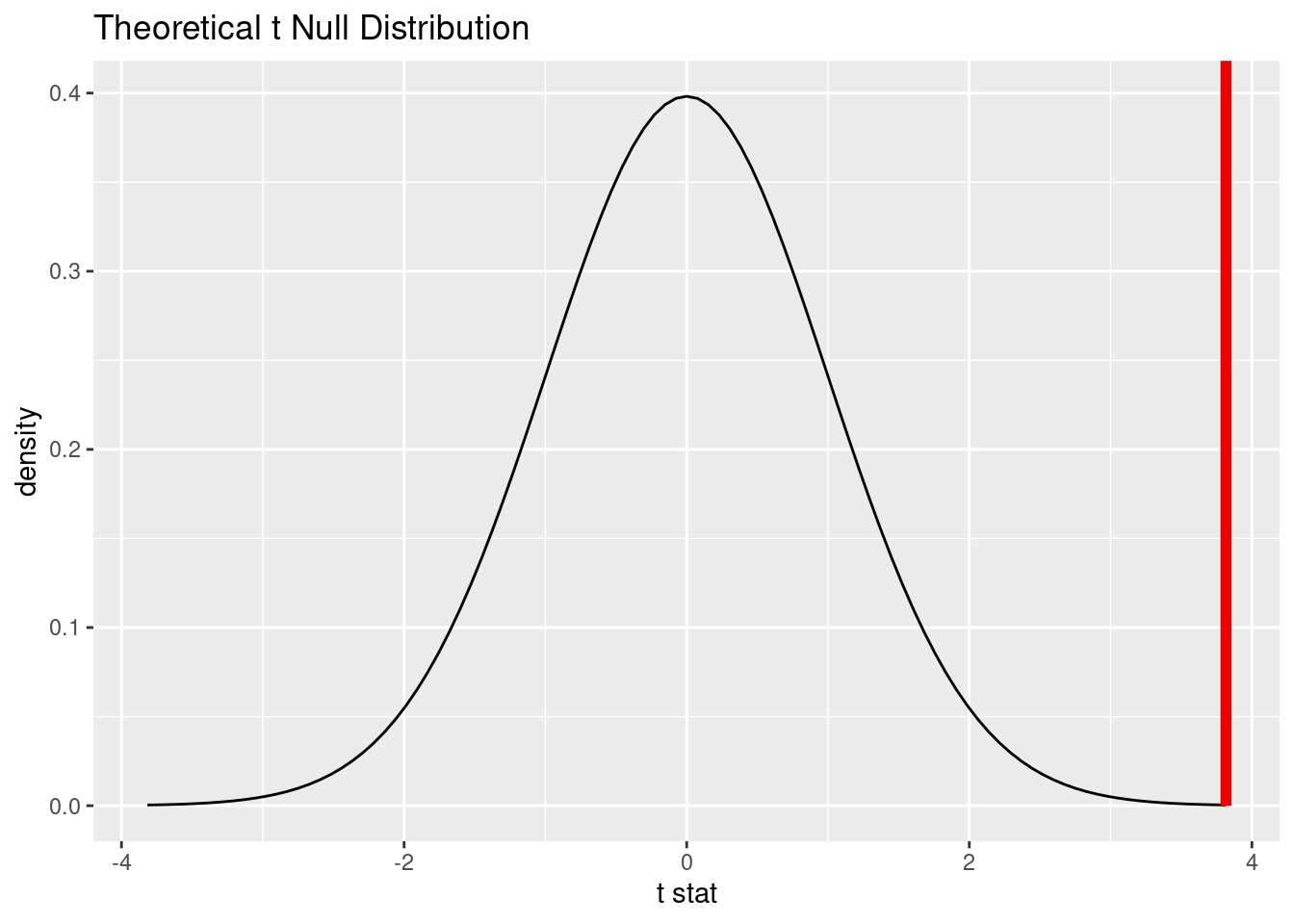
null_dist_theory|>
  get_p_value(obs_stat = t_hat, direction = "two-sided")
# A tibble: 1 × 1
p_value
<dbl>
1 0.000208