library(tidyverse)
library(openintro)
library(tidymodels)Inference for a mean
Warm up
Announcements
- No class tomorrow
- Lab 8 due Thursday
- Lab 9 optional
- Friday we will talk about final report formatting
Inference for one mean
Today’s focus
Inference for a population mean
Specifically, estimating a population mean via a confidence interval
And generally, what in the world is a confidence interval?!
Why is it constructed?
How is it constructed?
What do the bounds of a confidence interval mean?
What does the confidence level mean?
What is the margin of error?
Setup
Bootstrap confidence interval for the mean
Take a bootstrap sample (sample with replacement) of size n (the original sample size) from the original sample
Record the mean
Repeat steps 1 and 2 many times to build the bootstrap distribution
Find the bootstrap confidence interval using one of two methods:
Percentile method: The bounds of the middle X% of the bootstrap distribution comprise the X% bootstrap interval.
Standard error method:
Calculate the standard error for the bootstrap distribution
Find the critical value associated with the X% confidence interval
Calculate the margin of error (ME) as the critical value \(\times\) standard error
Construct the confidence interval a the original sample mean \(\pm\) ME
Case study: Length of gestation
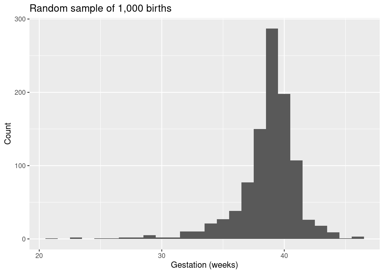
Every year, the United States Department of Health and Human Services releases to the public a large dataset containing information on births recorded in the country. This dataset has been of interest to medical researchers who are studying the relation between habits and practices of expectant mothers and the birth of their children. In this case study we work with a random sample of 1,000 cases from the dataset released in 2014. The length of pregnancy, measured in weeks, is commonly referred to as gestation. The histogram below shows the distribution of lengths of gestation from the random sample of 1,000 births.
ggplot(
  openintro::births14,
  aes(x = weeks)
  ) +
  geom_histogram(binwidth = 1) +
  labs(
    x = "Gestation (weeks)",
    y = "Count",
    title = "Random sample of 1,000 births"
  )
CS: Length of gestation - boot_dist
The distribution of bootstrapped means of gestation from 1,500 different bootstrap samples.
set.seed(1234)

boot_dist <- births14 |>
  specify(response = weeks) |>
  generate(
    reps = 1500,
    type = "bootstrap"
  ) |>
  calculate(stat = "mean")

visualize(boot_dist)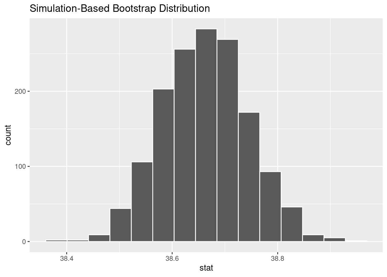
CS: Length of gestation - percentile interval
What does the following code do? How do you adjust it to change the confidence level?
boot_dist |>
  get_ci()
# A tibble: 1 × 2
lower_ci upper_ci
<dbl> <dbl>
1 38.5 38.8boot_dist |>
summarize(
lower = quantile(stat, 0.025),
upper = quantile(stat, 0.975)
)# A tibble: 1 × 2
lower upper
<dbl> <dbl>
1 38.5 38.8CS: Length of gestation - standard error interval
What does the following code do? Why do we need to provide point_estimate?
obs_stat <- births14 |>
  specify(response = weeks) |>
  calculate(stat = "mean")

obs_stat
Response: weeks (numeric)
# A tibble: 1 × 1
stat
<dbl>
1 38.7boot_dist |>
get_ci(
type = "se",
point_estimate = obs_stat,
level = 0.95
)# A tibble: 1 × 2
lower_ci upper_ci
<dbl> <dbl>
1 38.5 38.8Interpretations
The interval: (38.5, 38.8)
The confidence level: 95%
What does 95% confidence interval mean?
We are 95% confident that the true mean gestational period is between 38.5 and 38.8 weeks.
Bootstrap confidence intervals
Exercise 1
Construct and interpret a 95% confidence interval, using the standard error method with the get_ci() function, for the average length of gestation.
obs_stat <- births14 |>
  specify(response = weeks) |>
  calculate(stat = "mean")

obs_stat
Response: weeks (numeric)
# A tibble: 1 × 1
stat
<dbl>
1 38.7boot_dist |>
get_ci(
type = "se",
point_estimate = obs_stat,
level = 0.95
)# A tibble: 1 × 2
lower_ci upper_ci
<dbl> <dbl>
1 38.5 38.8Add response here.
Exercise 2
Construct the interval without using the get_ci() (or get_confidence_interval()) function.
# option 1 for se
se <- boot_dist |>
  summarize(se = sd(stat)) |>
  pull(se)

se
[1] 0.08122163# option 2 for se
sd(boot_dist$stat)[1] 0.08122163#option 1 for ci
obs_stat |>
mutate(lower = stat - 1.96*se,
upper = stat + 1.96*se)Response: weeks (numeric)
# A tibble: 1 × 3
stat lower upper
<dbl> <dbl> <dbl>
1 38.7 38.5 38.8# option 2 for ci
xbar = mean(births14$weeks)
c(xbar - 1.96*se, xbar + 1.96*se)[1] 38.50681 38.82519Exercise 3
Would you expect a 90% confidence interval for the average length of gestation to be wider or narrower? Explain your reasoning.
Exercise 4
Now construct a 90% confidence interval for the average length of gestation and confirm your answer from the previous exercise. Repeat as little of your code as possible.
boot_dist |>
  get_ci(
    type = "se",
    point_estimate = obs_stat,
    level = 0.90
  )
# A tibble: 1 × 2
lower_ci upper_ci
<dbl> <dbl>
1 38.5 38.8Confidence intervals with mathematical models
If technical conditions are satisfied, the distribution of the sampling mean (i.e., the sampling distribution) follows the t-distribution with n - 1 degrees of freedom, where n is the sample size.
sampling_dist <- births14 |>
  specify(response = weeks) |>
  assume(distribution = "t")

sampling_dist
A T distribution with 999 degrees of freedom.visualize(sampling_dist)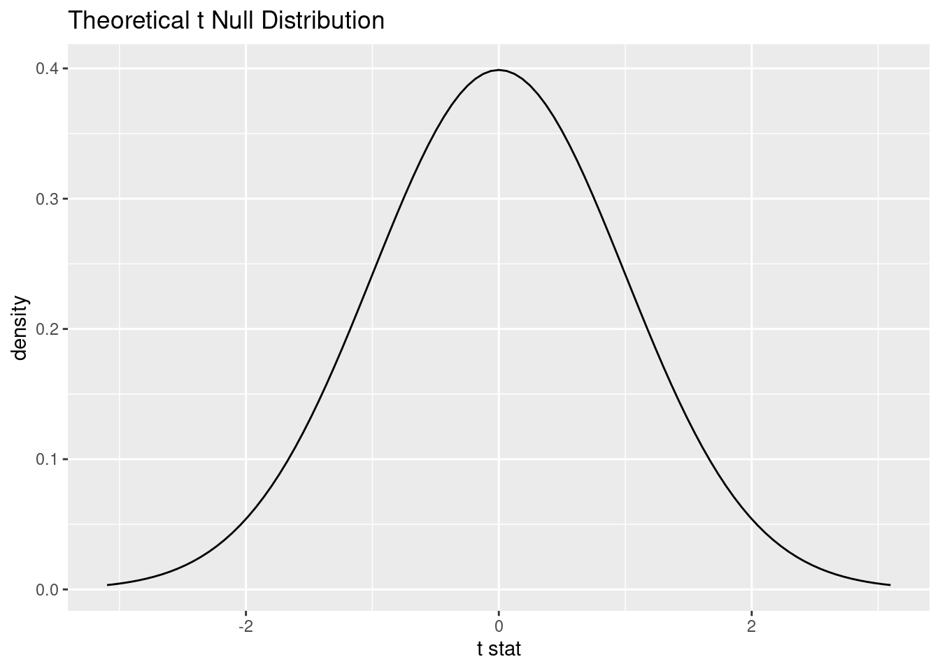
Exercise 5
Construct and visualize a confidence interval using mathematical models for the average length of gestation.
# option

 births14 |>
   specify(response = weeks) |>
   assume(distribution = "t") |>
   get_ci(type = "se", point_estimate =  obs_stat)
# A tibble: 1 × 2
lower_ci upper_ci
<dbl> <dbl>
1 38.5 38.8 #option 2
s <- sd(births14$weeks)
n <- nrow(births14)
se <- s/sqrt(n)
se[1] 0.08111118 # mathematical model ci approx N
# cv using normal
qnorm(0.975)[1] 1.959964# cv using t dist
qt(0.975, df = n-1)[1] 1.962341#our case: df is large, so both are about 1.96
c(xbar - 1.96*se, xbar + 1.96*se)[1] 38.50702 38.82498