library(tidyverse)
library(tidymodels)
library(scatterplot3d)Regression with multiple predictors
Warm up
Announcements
- No lab or class on Monday, May 27th.
- Project proposal due Tuesday, May 28th.
- Lab 3 due Wednesday, May 29th.
Load packages and data
\(R^2\) and model fit
\(R^2\)
\(R^2\), aka “the coefficient of determination” or “correlation squared” is a way to see how well a given model fits the data.
\[ R^2 = r^2 \]
Sum of squares total, SST
The sum of squares total is a measure of the total variability in the outcome variable:
\[ SST = (y_1 - \bar{y})^2 + (y_2 - \bar{y})^2 + \cdots + (y_n - \bar{y})^2 \]
Sum of squares residuals, SSE
The sum of squares residuals (error) is a measure of the variability in the residuals, i.e., variability left unexplained in the outcome variable after the model is fit:
\[ SSE = (y_1 - \hat{y}_1)^2 + (y_2 - \hat{y}_2)^2 + \cdots + (y_n - \hat{y}_n)^2 \]
\(R^2\), another look
\[ R^2 = \frac{SST - SSE}{SST} = 1 - \frac{SSE}{SST} \]
. . .
- This can be summarized as “\(R^2\) is 1 minus the sum of squared residuals divided by the sum of squared total”.
. . .
- In other words, \(R^2\) is the proportion of variability in the outcome that is explained by the model.
\(R^2\)
If the sum of squared residuals is 0, then the model explains all variability and \(R^2 = 1 - 0 = 1\).
If the sum of squared residuals is the same as all the variability in the data, then model does not explain any variability and \(R^2 = 1 - 1 = 0\).
\(R^2\) is a measure of the proportion of variability the model explains. An \(R^2\) of 0 is a poor fit and \(R^2\) of 1 is a perfect fit.
Finding \(R^2\)
To find \(R^2\) simply call the function glance() on your model_fit, e.g.
model_fit <- linear_reg() |>
  fit(outcome ~ predictor, data = data_set)

glance(model_fit)
Models with multiple predictors
Two predictors
\[ y = \beta_0 + \beta_1 x_1 + \beta_2 x_2 + \epsilon \]
- \(y\): the outcome variable. Also called the “response” or “dependent variable”. In prediction problems, this is what we are interested in predicting.
- \(x_i\): the \(i^{th}\) predictor. Also commonly referred to as “regressor”, “independent variable”, “covariate”, “feature”, “the data”.
- \(\beta_i\): “constants” or coefficients i.e. fixed numbers. These are population parameters. \(\beta_0\) has another special name, “the intercept”.
- \(\epsilon\): the error. This quantity represents observational error, i.e. the difference between our observation and the true population-level expected value: \(\beta_0 + \beta_1 x\).
- Effectively this model says our data \(y\) is linearly related to the \(x_1\) and \(x_2\) but is not perfectly observed due to unexplained errors.
A simple example
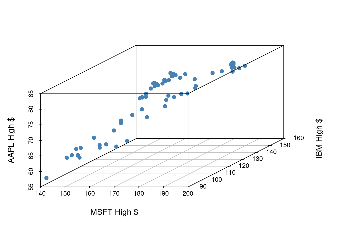
Let’s examine the first quarter of 2020 high prices of Microsoft, IBM, and Apple stocks to illustrate some ideas.

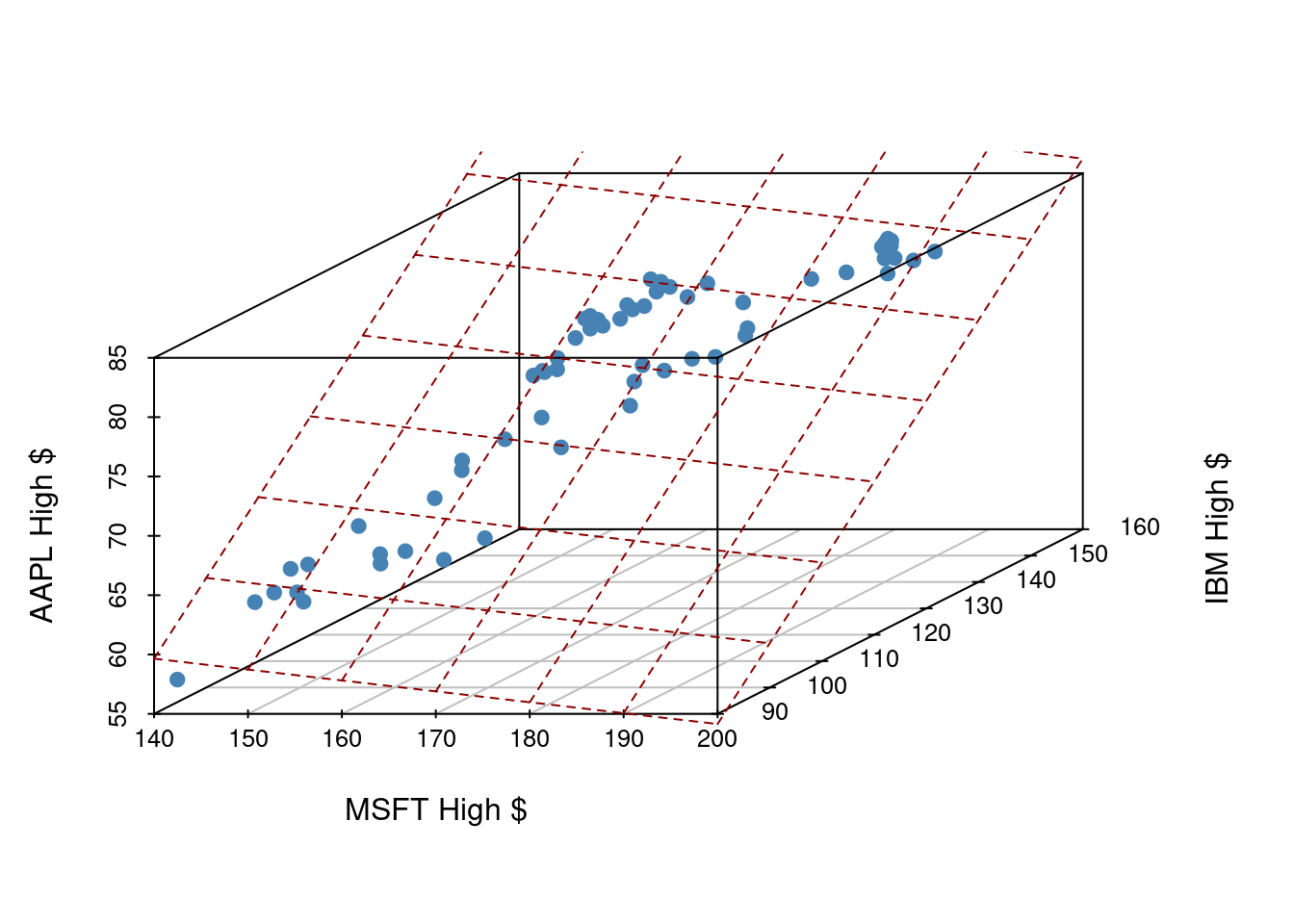
If we have three measurements (variables) then each observation is a point in three-dimensional space. In this example, we can choose one of our measurements to be the outcome variable (e.g. Apple stock price) and use our other two measurements (MSFT and IBM price) as predictors.
In general, the total number of measurements, i.e. variables (columns) in our linear model represents the spatial dimension of our model.
2 predictors + 1 outcome = 3 dimensions
The fitted linear model no longer looks like a line, but instead looks like a plane. It shows our prediction of AAPL price (\(y\)) given both MSFT price (\(x_1\)) and IBM price (\(x_2\)).

Fitting a multiple regression model in R
Find the equation of the plane by adding in new predictors:
my_model_fit <- linear_reg() |>
  fit(outcome ~ predictor1 + predictor2 + predictor3 + ..., data = data_frame)
. . .
- This code template will fit the model according to the ordinary least squares (OLS) objective function, i.e., we are finding the equation of the hyperplane that minimizes the sum of squared residuals
. . .
- You can then display a tidy output of the model with the
tidy()function on your fitted model:tidy(my_model_fit)
Today we’ll explore the question “How do volume and weights books relate?” and “How, if at all, does that change when we take whether the book is hardback or paperback into consideration?”
Goals
Build, fit, and interpret linear models with more than one predictor
Use categorical variables as a predictor in a model
Compute \(R^2\) and use it to select between models
Packages
library(DAAG)Data
The data for this application exercise comes from the allbacks dataset in the DAAG package. The dataset has 15 observations and 4 columns. Each observation represents a book. Let’s take a peek at the data:
allbacks volume area weight cover
1 885 382 800 hb
2 1016 468 950 hb
3 1125 387 1050 hb
4 239 371 350 hb
5 701 371 750 hb
6 641 367 600 hb
7 1228 396 1075 hb
8 412 0 250 pb
9 953 0 700 pb
10 929 0 650 pb
11 1492 0 975 pb
12 419 0 350 pb
13 1010 0 950 pb
14 595 0 425 pb
15 1034 0 725 pbNote that volume is measured in cubic centimeters and weight is measured in grams. More information on the dataset can be found in the documentation for allbacks, with ?allbacks.
Single predictor
Exercise 1
Visualize the relationship between volume (on the x-axis) and weight (on the y-axis). Overlay the line of best fit. Describe the relationship between these variables.
# add code hereAdd response here.
Exercise 2
Fit a model predicting weight from volume for these books and save it as weight_fit. Display a tidy output of the model.
# add code hereExercise 3
Interpret the slope and the intercept in context of the data.
Add response here.
Exercise 4
Calculate the \(R^2\) of this model and interpret it in context of the data.
# add code hereAdd response here.
Multiple predictors
Exercise 5
Visualize the relationship between volume (on the x-axis) and weight (on the y-axis), taking into consideration the cover type of the book. Use different colors and shapes for hardback and paperback books. Also use different colors for lines of best fit for the two types of books. In addition, add the overall line of best fit (from Exercise 1) as a gray dashed line so that you can see the difference between the lines when considering and not considering cover type.
# add code hereExercise 6
Fit a model predicting weight from volume for these books and save it as weight_cover_fit. Display a tidy output of the model.
# add code hereExercise 7
In the model output we have a variable coverpb. Why is only the pb (paperback) level of the cover variable shown? What happened to the hb (hardback) level?
Add response here.
Exercise 8
Interpret the slopes and the intercept in context of the data.
Add response here.
Exercise 9
First, guess whether the \(R^2\) of this model will be greater than, less than, or the same as the previous model, or whether we can’t tell. Then, calculate the \(R^2\) of this model to confirm your guess, and then interpret it in context of the data.
# add code hereAdd response here.
Exercise 10
Which model is preferred for predicting book weights and why?
Add response here.
Exercise 11
Using the model you chose, predict the weight of a hardcover book that is 1000 cubic centimeters (that is, roughly 25 centimeters in length, 20 centimeters in width, and 2 centimeters in height/thickness).
# add code here